Data Ingestion and Analysis

PIVA includes a continuously expanding library of analysis routines and procedures, which, along with detailed documentation, can be found in the module working_procedures. While the module can be imported and used in any environment of the user’s choice, the following example demonstrates how data ingestion and initial analysis can be performed using a Jupyter Notebook template and the export tools embedded in PIVA.

More details on exporting workspaces between the PIVA GUI and Jupyter Notebook can be found here.

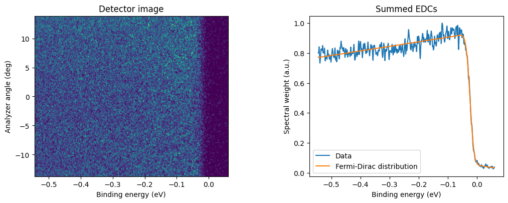
To provide step-by-step instructions, from loading the data file to displaying the fitting results, the following example demonstrates a generic case of determining the Fermi level correction and the experimental energy resolution based on a measurement of polycrystalline gold.

Presented example can be tested by downloading the data.

# import relevant packages

# piva packages
import piva.data_loaders as dl
import piva.working_procedures as wp

# general python utilities
import numpy as np
from matplotlib import pyplot as plt

# from matplotlib import interactive
import pandas as pd
# from scipy import optimize as opt

# use "matplotlib qt" to open plots in an interactive window
use_qt = False
if use_qt:
    %matplotlib qt
else:
    %matplotlib inline

# load file and extract data for easier access
path = "./"
fname = "Au-test_spectrum.p"
dataset = dl.load_data(path + fname)
data, slit_ax, erg_ax = dataset.data[0, :, :], dataset.yscale, dataset.zscale

Fit Fermi-Dirac Distribution

Plot the raw spectrum, prepare the data for analysis, and fit the Fermi-Dirac function using the fit_fermi_dirac method.

# plot and fit the measured scan
fig = plt.figure(figsize=[11, 4])
gs = fig.add_gridspec(
    1, 2, wspace=0.42, hspace=0.25, top=0.9, bottom=0.1, left=0.1, right=0.95
)
ax00 = fig.add_subplot(gs[0, 0])
ax01 = fig.add_subplot(gs[0, 1])

# display the detector image
ee, kk = np.meshgrid(erg_ax, slit_ax)

ax00.pcolormesh(ee, kk, data)
ax00.set_title("Detector image")
ax00.set_xlabel("Binding energy (eV)")
ax00.set_ylabel("Analyzer angle (deg)")


# analyze the data
edc = wp.normalize(np.sum(data, axis=0))  # summarize all angular channels
ε0 = erg_ax[wp.detect_step(edc)]  # find initial guess for E_F

res = wp.fit_fermi_dirac(
    erg_ax, edc, ε0, T=dataset.temp
)  # fit Fermi-Dirac distrubution with a Gausian component
par, fit_func, cov, resol, Δresol = res  # extract fitting results
Fermi_Dirac = fit_func(erg_ax)  # get the Fermi-Dirac distribution

# plot the summed EDC and the fitted curve
ax01.plot(erg_ax, edc, label="Data")
ax01.plot(erg_ax, Fermi_Dirac, label="Fermi-Dirac distribution")
ax01.set_title("Summed EDCs")
ax01.set_xlabel("Binding energy (eV)")
ax01.set_ylabel("Spectral weight (a.u.)")
ax01.legend();

Fit results

Display the fit results for comparison.

Ef = "{:.2f}".format(par[0] * 1000)
ΔEf = "{:.2f}".format(np.sqrt(np.diag(cov)[0]) * 1000)
σ = "{:.2f}".format(resol * 1000)
Δσ = "{:.2f}".format(Δresol * 1000)

df = {
    "scan name": [fname],
    "Ef, meV": [Ef],
    "Ef error, meV": [ΔEf],
    "resolution, meV": [σ],
    "resolution error, meV": [Δσ],
}
df = pd.DataFrame(data=df)
df

	scan name	Ef, meV	Ef error, meV	resolution, meV	resolution error, meV
0	Au-test_spectrum.p	-23.49	0.24	25.01	0.82

Contributing

We encourage everyone to share their tested, self-written analysis and modeling procedures with the community by adding them to PIVA’s source code. This can be done ideally directly through GitHub or alternatively by contacting the development team:

Wojtek Pudelko and Kevin Kramer